Two physical quantities need to be measured in this experiment.
The volume of a fixed amount of atmospheric air is measured as a function
of temperature at fixed pressure.
The temperature is varied with the use of
hot water is the second measurable.
Make the following table in your
notebook and fill in the details.
|
S. No. |
Physical quantity |
Independent / Dependent parameters |
Measured with |
Measuring instrument’s |
||
|
Minimum |
Maximum |
Least count |
||||
|
1 |
Temperature |
|
|
|
|
|
|
2 |
Volume |
|
|
|
|
|
How to measure Volume:
-
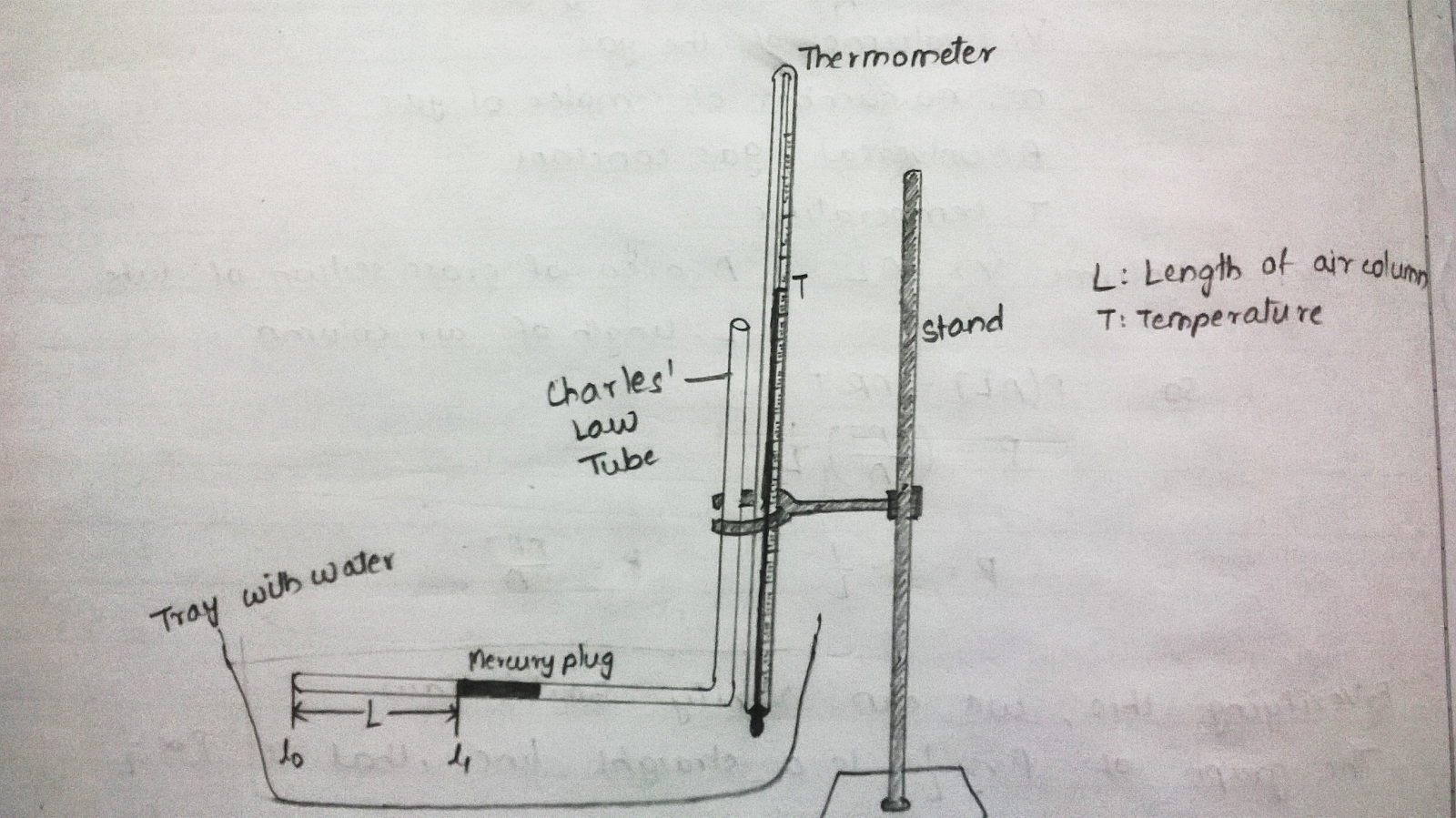
The volume of gas is enclosed in a (almost) cylindrical tube. (Neglect the curvature of the closed tube and the surface of mercury).
-
Hence the volume is . Here L = \(l_{1}\)- \(l_{0}\) (as shown in the figure below).
-
As Cross section is constant and volume is proportional to L, take readings for volume in terms of L.
-
Charles’ Law tube:
-
Make sure that the mercury plug is intact. If it is not there, bring all the mercury to form a single plug by gently hitting the tube.
-
Set up the apparatus, such that the horizontal portion of Charles’ Law tube apparatus is few mm above the tray surface, completely immersed in water and parallel to water level.
-
Fix a thermometer in vertical position with its bulb just above the tray surface.
-
-
Travelling microscope:
-
Focus the travelling microscope to clearly see the mercury bulb in the horizontal portion of Charles’ Law tube.
-
Make sure that the horizontal sides of the tray and the travelling microscope are parallel to each other.
-
Now, move the travelling microscope horizontally (using the screw) to clearly see the end of the horizontal tube. Note this reading as \(l_{0}\).
-
-
Heat water in an electric kettle until it boils.
-
Pour the hot water into the tray. (Note: Warm up the pan by first rinsing it with hot water.) Enough water should be in the tray to submerge the horizontal portion of Charles’ Law tube apparatus, yet leave a portion of the end beyond the bend above the water surface
-
Now focus the travelling microscope to the meniscus of the mercury plug facing the closed end of the Charles’ Law Tube. Note down the horizontal scale reading of the travelling microscope as \(l_{1}\).
-
Simultaneously read the temperature of the water in the tray. Record this as \(T\). And note down the time. Record these values in Table II.
-
While continuously observing the temperature of the water in the tray record temperature and column length as described above at approximately 5 to 100 C intervals as the temperature falls.
-
Plot the following Graphs
-
Temperature (T) vs - Volume (L)
-
Time (t) vs - Temperature (T)
-
-
Perform the least square fitting of the data in graph A to a straight line –
$$L = mT + c$$ (Remember L represents volume)
The temperature for which the volume goes to 0 corresponds to absolute zero.
$$0 = mT + c$$
Absolute temperature $$T=-cm$$
Also, extrapolate the fitted line and find out the absolute temperature as the temperature at which the straight line meets the temperature axis.
-
Perform the least square fitting of the data in graph B to and exponential decay. The same graph can be plotted as ln(t) vs Temperature and fit then fit to a straight line.
(This Graph and analysis has no implication to the Charles’s verification. This is the cooling curve of the water. Aim here is to see if the cooling can be described by Newton’s law of cooling.)
|
S.No. |
Time |
Temperature |
Length(\(l_{1}\)) |
volume |
||
|
\(MSR\) |
\(VSR\) |
\(MSR\)+\(VSR\)*\(LC\) |
\(L\)=\(l_{1}\)-\(l_{0}\) |
|||
|
|
Mins. |
C |
cm |
|
cm |
cm |
|
1 |
|
|
|
|
|
|
|
2 |
|
|
|
|
|
|
|
… |
|
|
|
|
|
|
|
… |
|
|
|
|
|
|
|
… |
|
|
|
|
|
|
|
10 |
|
|
|
|
|
|